OpFlowLab’s graphical user interface
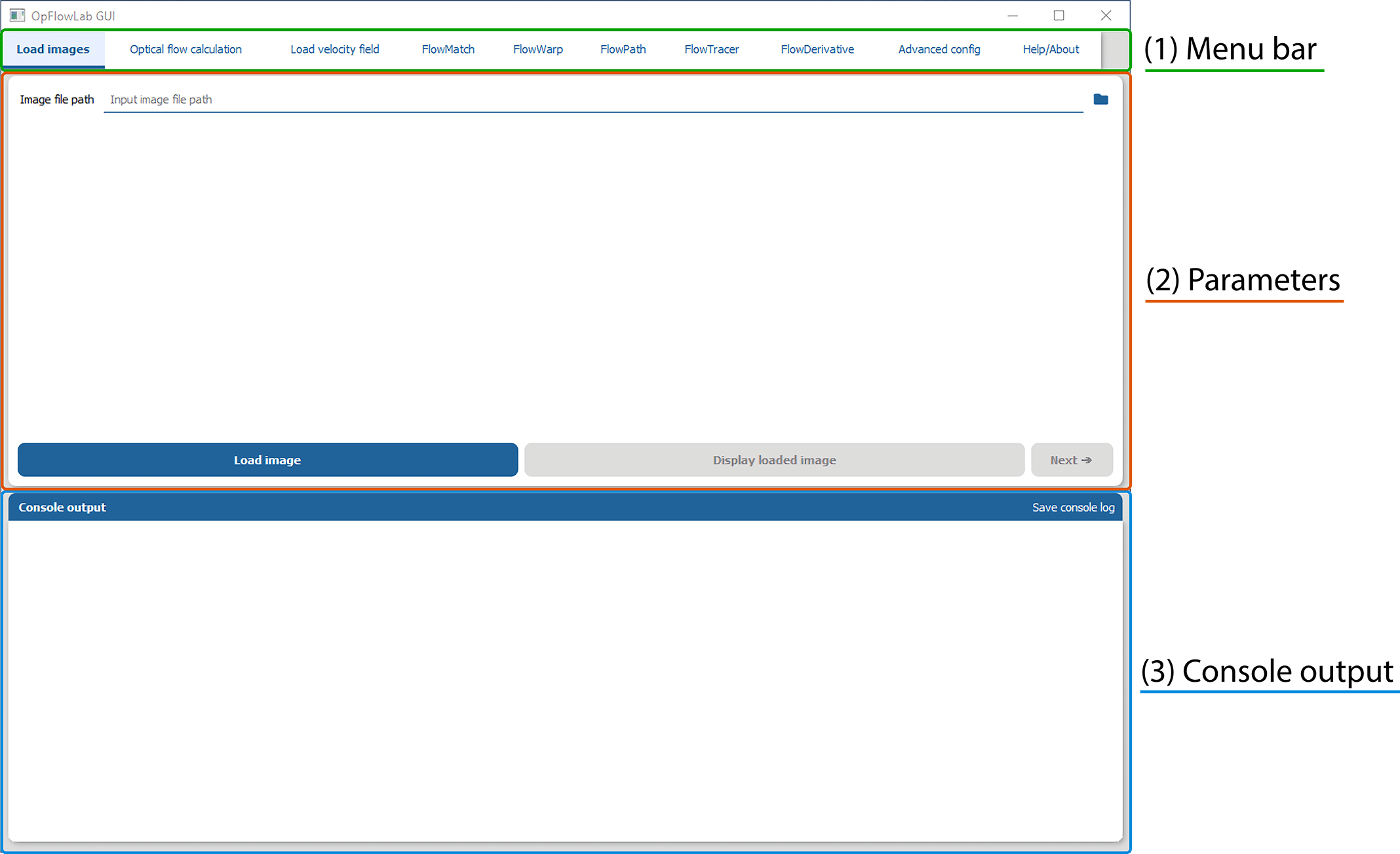
Menu bar — Allows for the selection of the various routines in the workflow.
Parameters — Allows for the selection of parameters for each routine in the workflow.
Console output — Shows the output generated from each routine. The console log can be saved by clicking the button labelled “Save console log”.
Loading images
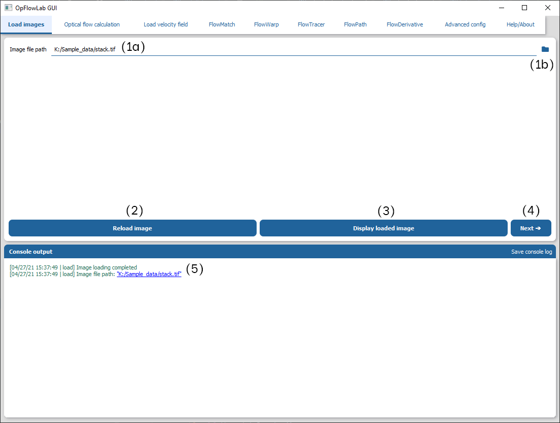
(a) Input box to key in path to image stack. (b) Opens a dialog box to select the image stack that is to be analysed.
Loads the image stack.
Displays the loaded image stack. Enabled only when an image stack has been loaded.
Moves to the next tab (Optical flow calculation). Enabled only when an image stack has been loaded.
Console output indicating the file that has been loaded.
Attention
Currently supported image types: *.tif.
Please ensure that this tiff image is a single image stack with all the time frames to be analysed.
Go to workflow: Loading images
Optical flow calculations
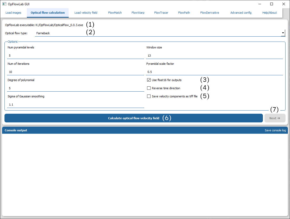
Location of the optical flow executable. Please ensure that this path is valid under the “Advanced config” tab.
Selects the optical flow algorithm to use.
Save each vector using a float16 format instead of a float32 format. The effect on precision should be minimal but provides a significant improvement in vector field saving and loading whilst saving disk space.
When checked, performs optical flow calculation in the reverse image stack order (reverse time direction).
When checked, saves the velocity files as a tif image instead of a binary file.
Calculates the velocity field using the specified optical flow algorithm.
Moves to the next tab (Load velocity field). Enabled only when the optical flow calculations are completed.
Tip
Determining the optimal set of parameters?
Determining the optimal set of parameters can be challenging as it is generally problem dependent. The default settings can serve as a good starting point to try out the various algorithms. However, we strongly recommend that a parameter search be done to determine the optimal parameters. We have provided an implementation of a grid search in OpFlowLab but other search algorithms can be used instead to speed up the time taken to determine the optimal parameters.
Farneback optical flow
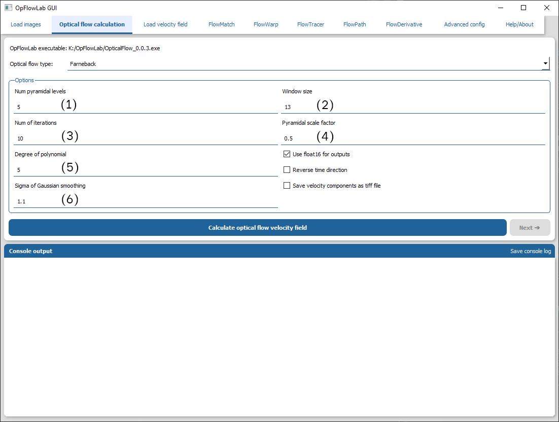
Specifies the number of pyramid levels to use.
Specifies the averaging window size that is used to reduce noise in the velocity field at the expense of a smoother field.
Specifies the number of iterations to perform per pyramid level to refine the velocity field.
Specifies the amount to scale the image for each pyramid level.
Specifies the size of the pixel neighbourhood used in polynomial expansion.
Specifies the standard deviation of the Gaussian applicability function.
Dense Pyramidal Lucas Kanade optical flow
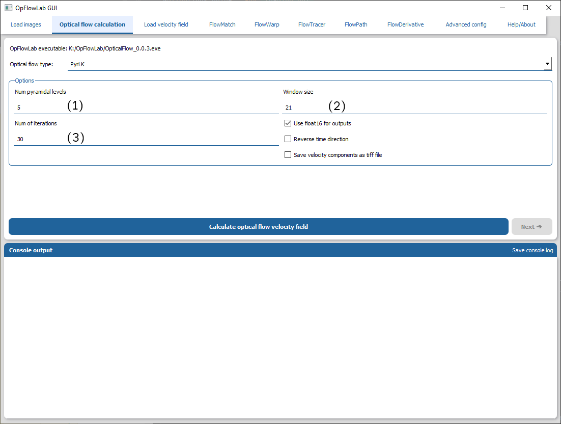
Specifies the number of pyramid levels to use.
Specifies the pixel neighbourhood to calculate the least square estimated of velocity for each pixel.
Specifies the number of iterations to perform per pyramid level to refine the velocity field.
Nvidia hardware optical flow
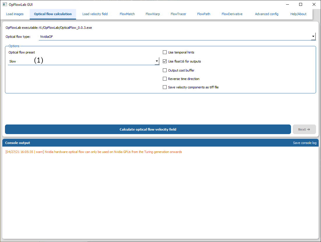
Specifies the preset used in calculating the velocity field.
Go to workflow: (1) Optical flow calculations
Load velocity fields
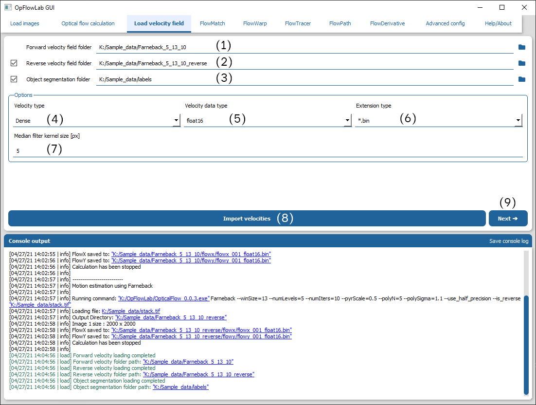
Specifies the folder containing the forward time direction velocity field.
When checked, specifies the folder containing the reverse time direction velocity field.
When checked, specifies the folder containing the labelled images.
Specifies if the velocity field is dense (1 velocity per pixel) or sparse (1 velocity per window).
Specifies if the velocity field is in the float16 or float32 format.
Specifies the extension of the velocity field.
Specifies if the neighbourhood size of the median filter. Set to None to not perform median filtering.
Loads the respective folders.
Moves to the next tab (FlowMatch).
Go to workflow: Load velocity field
(2) FlowMatch
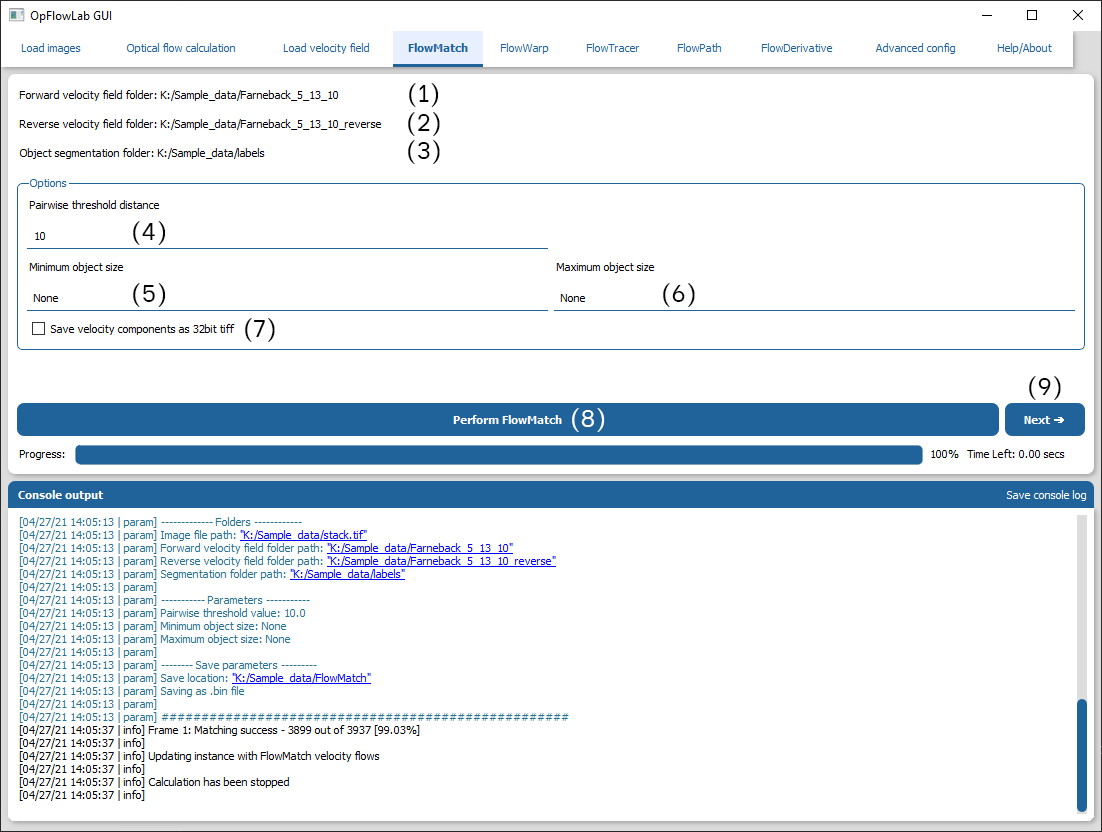
Location of the forward velocity fields. Please ensure that this path is valid under the “Load velocity field” tab.
Location of the reverse velocity fields. Please ensure that this path is valid under the “Load velocity field” tab.
Location of the labelled images. Please ensure that this path is valid under the “Load velocity field” tab.
Specifies the threshold used to determine valid pairs. This should be in the same order of magnitude (in pixels) of the movement.
Specifies the minimum size of the object that should be included in the FlowMatch process. Set to “None” to ignore.
Specifies the maximum size of the object that should be included in the FlowMatch process. Set to “None” to ignore.
Specifies if the vectors should be saved as a 32 bit tiff image instead of a binary file. (Not recommended)
Performs FlowMatch with the parameters specified above.
Moves to the next tab (FlowWarp).
Go to workflow: (2) FlowMatch – Object matching
(3a) FlowWarp
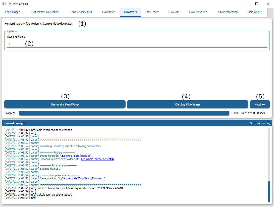
Location of the forward velocity fields. Please ensure that this path is valid under the “Load velocity field” tab.
Specifies the starting frame to perform the FlowWarp routine from. Used when multiple time frames are loaded.
Generates FlowWarp images with the parameters specified above.
Displays the FlowWarp image in a separate window.
Moves to the next tab (FlowTracer).
Go to workflow: (3a) FlowWarp – Velocity field validation
(3b) FlowTracer

Location of the forward velocity fields. Please ensure that this path is valid under the “Load velocity field” tab.
Location of the labelled images. Please ensure that this path is valid under the “Load velocity field” tab if “Object centroid” is used to generate the tracer locations.
Specifies the method used to generate the initial tracers.
Specifies if the initial tracer positions should be saved alongside the FlowTracer images.
Specifies the number of tracers to generate. This is only enabled when “Random tracers” is selected.
Specifies the distance between grid points used to generate the tracers. This is only enabled when “Grid tracers” is selected.
Performs FlowTracer with the parameters specified above.
Displays the FlowTracer image in a separate window.
Moves to the next tab (FlowPath).
Go to workflow: (3b) FlowTracer – Velocity field validation
(4) FlowPath
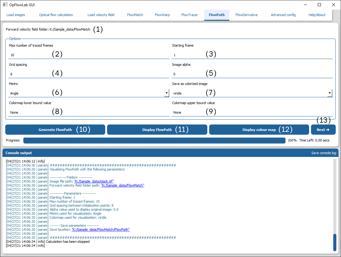
Location of the forward velocity fields. Please ensure that this path is valid under the “Load velocity field” tab.
Specifies the maximum number of frames that will be used to draw each path in the FlowPath image.
Specifies the starting frame to perform the FlowPath routine from. Used when multiple time frames are loaded.
Specifies the distance between grid points used to initialize the starting positions of the FlowPaths.
Specifies the alpha value of the FlowPath image. This produces an image showing the FlowPath as an overlay over the original image. Set to “None” to just output the FlowPath image.
Specifies the metric used to colourise the FlowPath image.
Specifies the colour map used to colourise the FlowPath image.
Specifies the lower bound of the colour map. Set to “None” to use the minimum value of the image.
Specifies the upper bound of the colour map. Set to “None” to use the maximum value of the image.
Performs FlowPath with the parameters specified above.
Displays the FlowPath image in a separate window.
Displays the colour map used to generate the image.
Moves to the next tab (FlowDerivative).
Go to workflow: (4) FlowPath – Velocity field visualization
(5) FlowDerivative
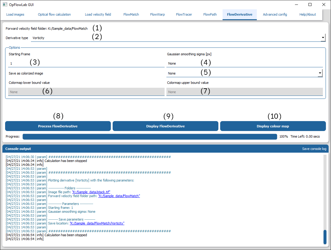
Location of the forward velocity fields. Please ensure that this path is valid under the “Load velocity field” tab.
Specifies the derivative that should be calculated from the velocity field.
Specifies the starting frame to perform the FlowDerivative routine from.
Specifies the sigma of the gaussian smoothing function. This should be set to a value 2x the average distance between objects.
Specifies the colour map used to colourise the FlowPath image.
Specifies the lower bound of the colour map. Set to “None” to use the minimum value of the image.
Specifies the upper bound of the colour map. Set to “None” to use the maximum value of the image.
Performs FlowDerivative with the parameters specified above.
Displays the FlowDerivative image in a separate window.
Displays the colour map used to generate the image.
Go to workflow: (5) FlowDerivative – Velocity field derivatives
Advanced config
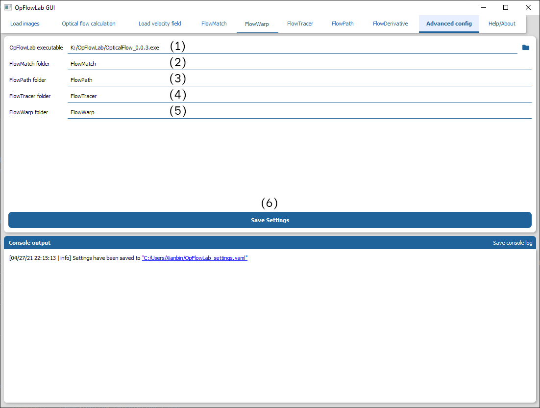
Input to specify the Location of the optical flow executable.
Specify the name of the folder to create for the FlowMatch routine.
Specify the name of the folder to create for the FlowWarp routine.
Specify the name of the folder to create for the FlowPath routine.
Specify the name of the folder to create for the FlowTracer routine.
Saves the configuration to a YAML file in the user’s home directory.