Workflow for OpFlowLab¶

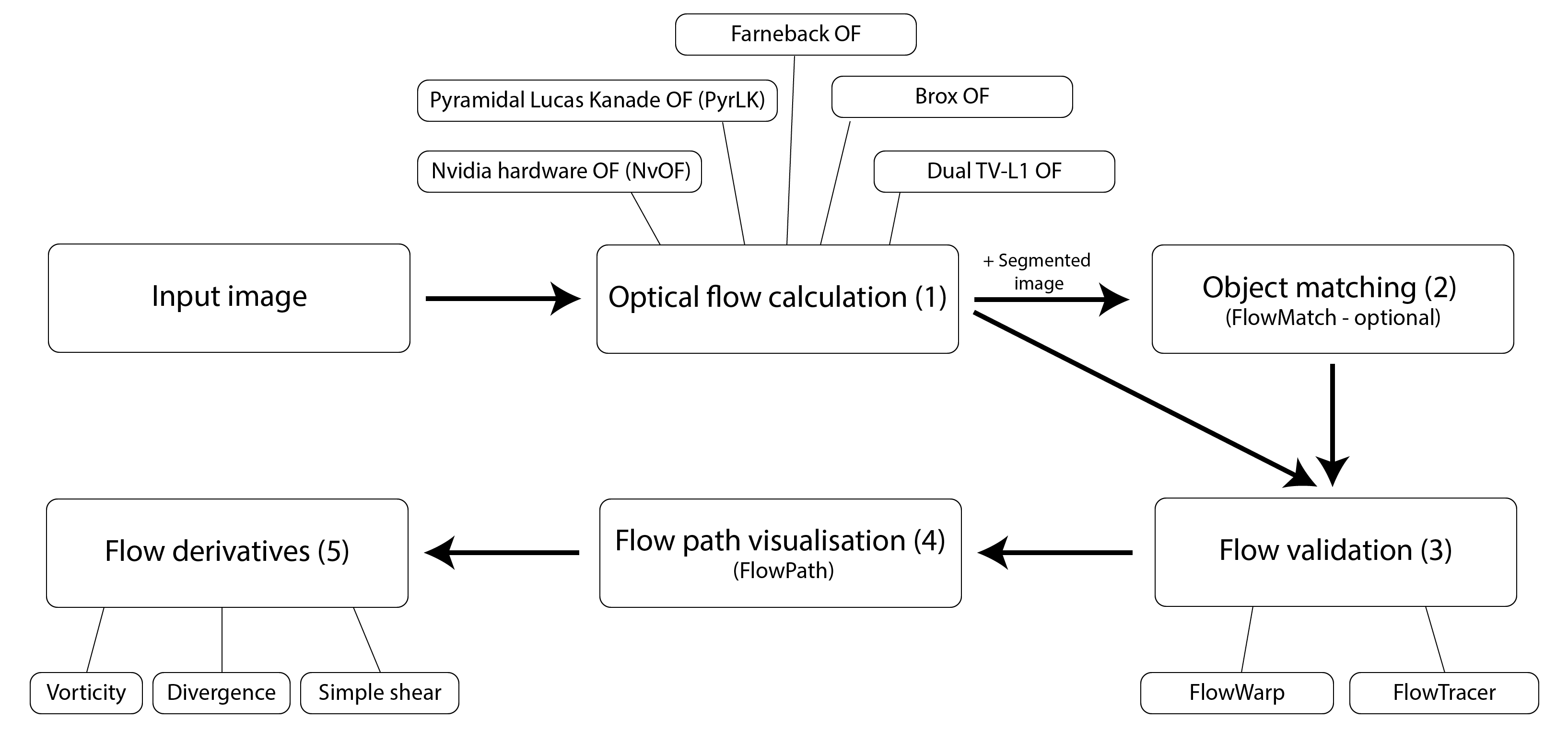
A typical workflow for OpFlowLab is shown above.

Tip

A YAML file (can be opened in any text editor) is created in the directory of the loaded image file. It lists the actions taken during each session. This will help you to trace your steps at a later time point if needed.

In addition, the text in the console can be saved at any time by pressing the text labelled “Save console log”.

Loading images¶

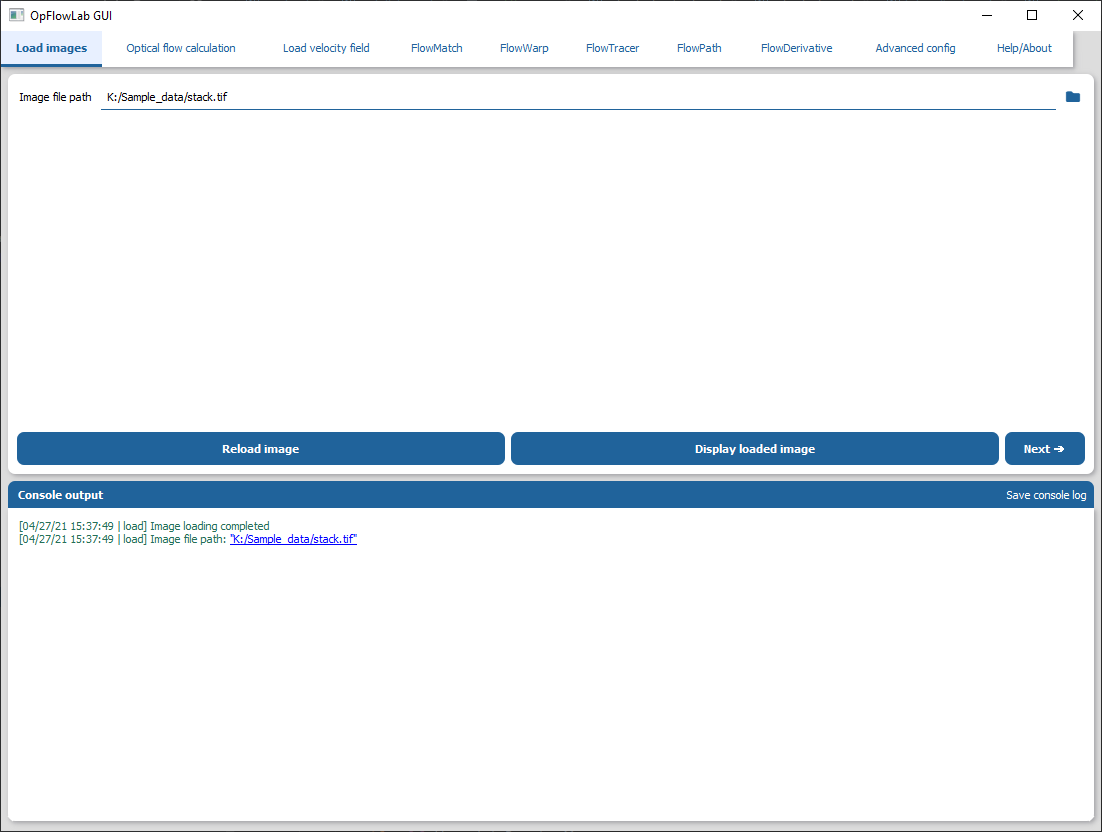
GUI/options guide: Loading images

Loading a single tif image containing multiple time slices:

Load the image into OpFlowLab either by inputting the path into the input box or select the directory icon and locate the file in your directory.
Press the “Load image” button (or “Reload image” if an image has been previously loaded).
There should be a confirmation that the image is loaded in the console.
You can verify that the image is loaded properly by pressing the “Display loaded image” button.
Press the ‘Next’ button when you are ready to move to the next step.

(1) Optical flow calculations¶

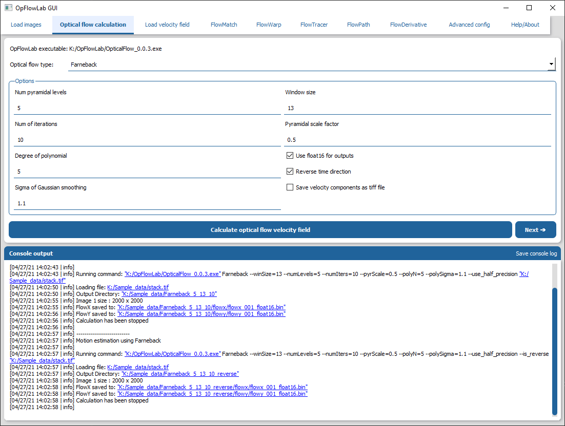
GUI/options guide: Optical flow calculations

Performing optical flow calculations in the forward time direction:

Ensure that the path to the OpFlowLab executable is correct.
Select the optical flow algorithm to use from the dropdown menu. See Choosing the right optical flow algorithm?.
Perform the optical flow calculations by pressing the button ‘Calculate optical flow velocity field’.
When the optical flow calculations are done press the ‘Next’ button.

Performing optical flow calculations in the reverse time direction:

Ensure that the “Reverse time direction” checkbox is selected.
Perform the same steps as when calculating velocities in the forward time direction.

Tip

Choosing the right optical flow algorithm?

The choice of optical flow algorithm is important to ensure that the velocity field is as accurate as possible. We recommend trying NvidiaOF on your dataset first if your hardware satisfies the requirements (see Setting up OpFlowLab for optical flow calculations (Windows)). If not, using the default settings for Farneback would also serve as a good starting point.

Load velocity field¶

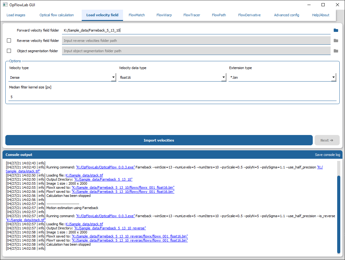
GUI/options guide: Load velocity fields

Select the forward velocity field folder:

Input the path in the text box labelled “Forward velocity field folder” or select the folder containing the velocity field calculated in (1). This folder should contain the folders “flowx” and “flowy”.

Select the reverse velocity field folder:

Check the checkbox labelled “Reverse velocity field folder”.
Input the path in the text box beside it or select the folder containing the velocity field calculated in (1). This folder should contain the folders “flowx” and “flowy”.

Select the object segmentation folder:

Check the checkbox labelled “Object segmentation folder”.
Input the path in the text box beside it or select the folder containing the labeled image. This folder should contain labeled images with each object assigned a unique value

Load the folders

Press the “import velocities” button.
There should be a confirmation that the folders are loaded in the console.

Tip

What folders should be loaded?

Not all folders are needed for certain routine. Below are the list of required folders for each routine:

FlowMatch – Image folder, forward velocity folder, reverse velocity folder and object segmentation folder
FlowWarp – Image folder and forward velocity folder
FlowTracer – Image folder and forward velocity folder. Object segmentation folder is needed if the “object centroids” option is selected
FlowPath – Image folder and forward velocity folder
FlowDerivative – Image folder and forward velocity folder

(2) FlowMatch – Object matching¶

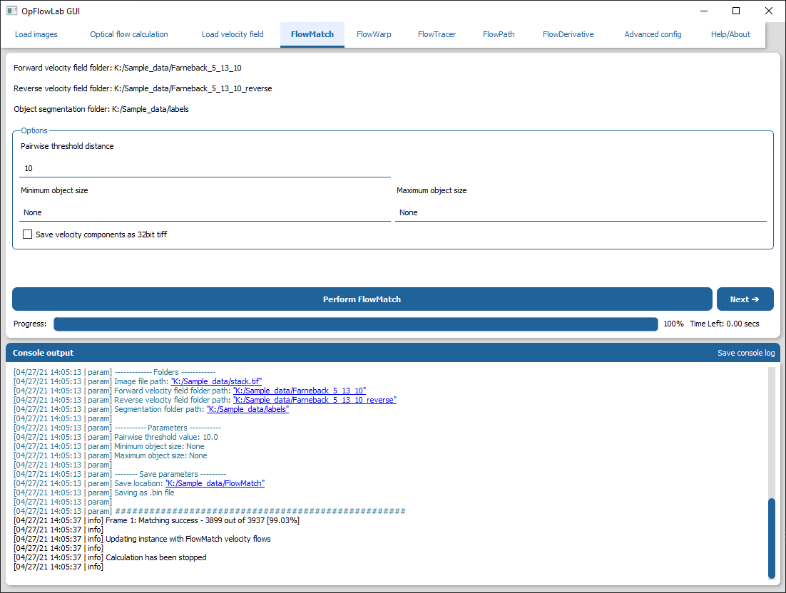
GUI/options guide: (2) FlowMatch

Perform object matching using the FlowMatch routine:

Ensure that the forward velocity, reverse velocity, and object segmentation folders are loaded.
The default values are a good starting point for object matching.
Run FlowMatch by pressing the “Perform FlowMatch” button.
The matched velocity is saved in a new “FlowMatch” folder in the directory with the loaded image file.
When the FlowMatch is done press the ‘Next’ button to move to velocity field validation using FlowWarp.

(3a) FlowWarp – Velocity field validation¶

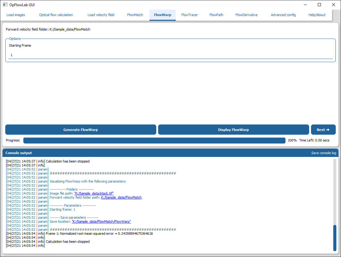
GUI/options guide: (3a) FlowWarp

Perform vector field validation using the FlowWarp routine:

Ensure that the forward velocity folder is loaded.
Run FlowWarp by pressing the “Generate FlowWarp” button.
The output for FlowWarp can be visualised by pressing the “Display FlowWarp” button.
The image file can be found in a new “FlowWarp” folder in the forward velocity directory.

(3b) FlowTracer – Velocity field validation¶

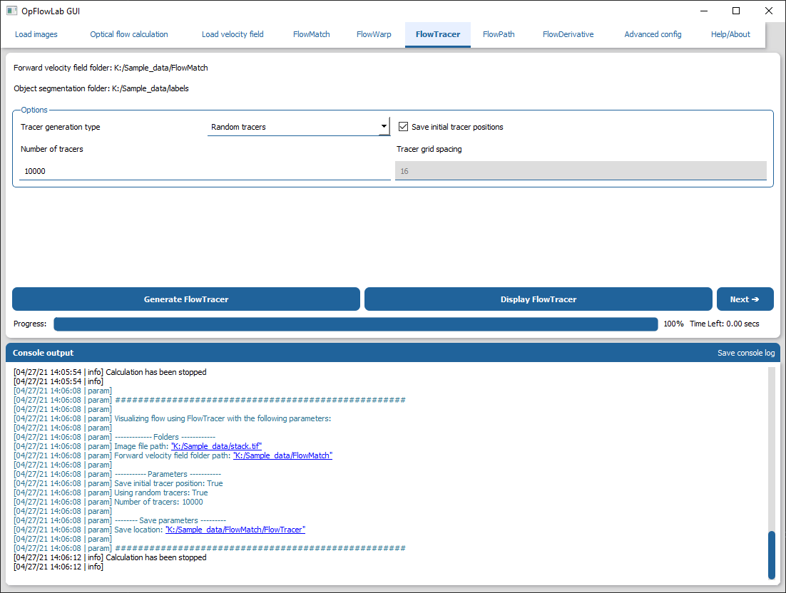
GUI/options guide: (3b) FlowTracer

Perform vector field validation using the FlowTracer routine:

Ensure that the forward velocity folder is loaded.
Select the type of tracer to generate by clicking the dropdown menu beside “Tracer generation type”. The types of initial tracers are as follows:
- Random tracers – Sets the initial location of tracers to a random location.
- Grid tracers – Set the initial location of the tracers based on a grid of a specified distance.
- Object centroids – Sets the initial location of tracers to the centroids of the objects in the image. If this is selected, please ensure the object segmentation folder is loaded.
Run FlowTracer by pressing the “Generate FlowTracer” button.
The output for FlowTracer can be visualised by pressing the “Display FlowTracer” button.
The image file can be found in a new “FlowTracer” folder in the forward velocity directory.

(4) FlowPath – Velocity field visualization¶

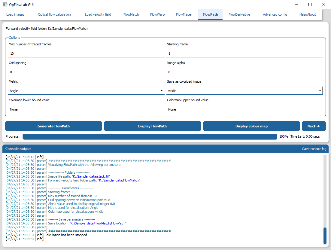
GUI/options guide: (4) FlowPath

Perform vector field visualization using the FlowPath routine:

Ensure that the forward velocity folder is loaded.
By default, the path will be colorized based on the average angle of the path using the viridis colormap
Run FlowPath by pressing the “Generate FlowPath” button
The output for FlowPath can be visualised by pressing the “Display FlowPath” button.
The image file and colour map can be found in a new “FlowPath” folder in the forward velocity directory.

(5) FlowDerivative – Velocity field derivatives¶

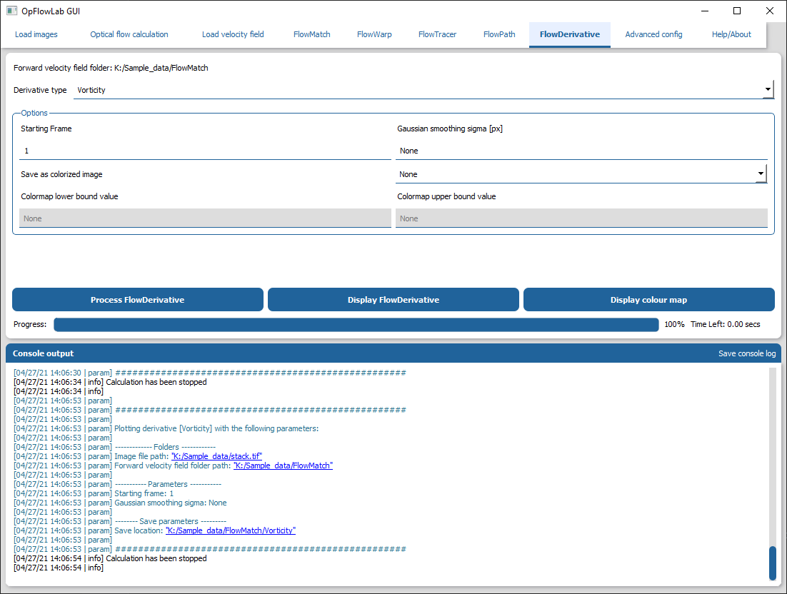
GUI/options guide: (5) FlowDerivative

Calculate vector field derivatives using the FlowDerivative routine:

Ensure that the forward velocity folder is loaded.
Select the type of derivative to be calculated using the “Derivative type” drop down menu
Run FlowDerivative by pressing the “Process FlowDerivative” button
The output for FlowDerivative can be visualised by pressing the “Display FlowDerivative” button.
The image file and colour map can be found in a new folder labelled with the derivative type in the forward velocity directory.